LP Estimated Diffuse Signal Approach to Blind Microphone Geometry Calibration
Methodology
Step-1
Reverberant speech signal is decomposed into the constituent early and late components. $$x_m[n]=x_{m,e}[n]+x_{m,l}[n],~\forall~m$$ Weighted prediction error (WPE) method, which is typically used for speech deverberation is used for the signal decomposition.Step-2
Late component exhibits diffuse noise properties, which has a distance cue. Spatial cross coherence function of the late part is used to estimate the microphone separation.Spatial cross coherence function is computed as, $$ \Gamma_{ij}[k]=\frac{\mathbb{E}\{X_{i,l}[k]X_{j,l}^*[k]\}}{\sqrt{\mathbb{E}\{|X_{i,l}[k]|^2\}\mathbb{E}\{|X_{j,l}[k]|^2\} }}$$ where \(X_{i,l}[k]\) is the Fourier transform of \(x_{i,l}[n]\). For a spherically isotropic diffuse noise field, $$ \Gamma_{ij}^s[k]=sinc \left (\frac{2\pi k f_s d_{ij}}{Kc} \right )$$ \(\Gamma_{ij}[k]\) is matched against \(\Gamma_{ij}^s[k]\) for the estimation of distance between microphone pair \(i,j\) $$d_{ij}=\underset{d_{ij}}{\arg\min}~\sum_{k=0}^{K/2} |\Gamma_{ij}[k]-\Gamma_{ij}^s[k]|^2 $$
Step-3
Given estimates of distances between all pairs of microphones, Multi-dimensional scaling (MDS ) is used to estimate the microphone geometry.Illustration
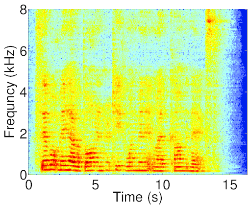
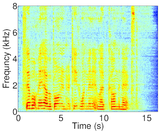
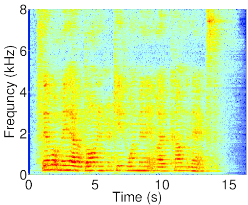
Signal decomposition
Real data experiments
Lab recording example
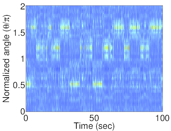
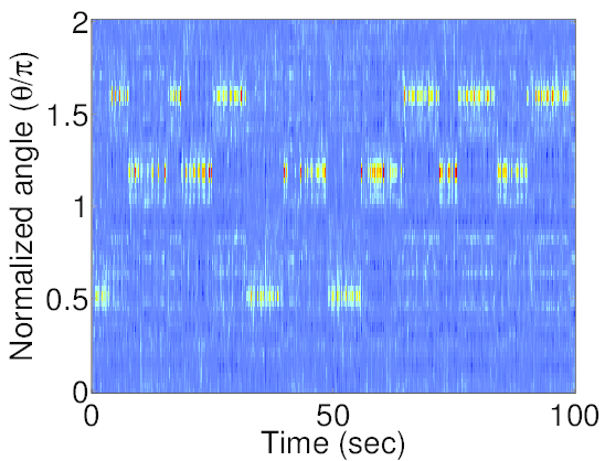
The synthetic meeting recording has a conversation between three participants. Spatial response using estimated microphone geometry is noisy compared to that obtained using the original geometry. However, the locations of peaks are in agreement.
AMI meeting corpus example [link]
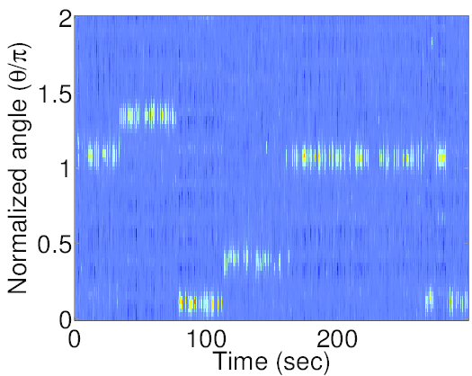

The meeting recording has a conversation between four participants in a conference room at Edinburgh (ES2016a). The response shows the speaker activity as a function of time. Spatial response using estimated microphone geometry closely matches that obtained using the original geometry
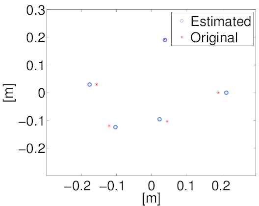
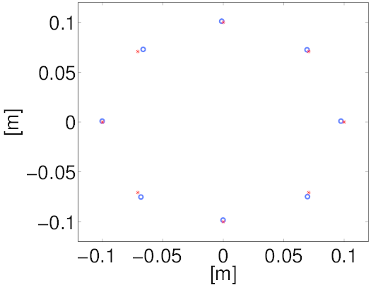
Framewise geometry estimation
The distance estimates obtained in each frame are used to estimate the geometry of microphones. The geometry estimates from each frame are rotated such that the origin is at the geometric center, first microphone is along the \(x\)-axis and the second microphone is in the positive \(x-y\) plane. Animation below shows the geometry estimates for each frame. (Shown in red is the original microphone geometry)